Log-t distribution

The log-t distribution models the uncertainty about positive-valued quantities that follow a log-normal distribution with unknown mean and standard deviation. If the values of log-transformed measurements/observations follow a Normal distribution and the Normal-gamma distribution is used as a conjugate prior to learn the mean and precision of the Normal distribution, then the predictive distribution for the original (i.e., not transformed) measurements follows a log-t distribution.

When working with the log-t distribution, one should be aware that it does not have a finite mean or a finite variance.

Definition

Let $Y$ follow a Student's t-distribution with $\eta$ degrees of freedom. Then, $X$, $$
X = \exp\left( \gamma + \tau \cdot X \right)\;,
$$ follows a log-t distribution with parameters $\gamma$, $\tau$ and $\eta$. 

The probability density function (PDF) of the log-t distribution can be expressed in terms of the PDF $f_{t_\eta}(y)$ of the Student's t-distribution with $\eta$ degrees of freedom: $$
f(x|\gamma,\tau,\eta) = \frac{1}{x\cdot \tau}\cdot f_{t_\eta}\left(\frac{\ln(x)-\gamma}{\tau}\right)\;.
$$

Equivalently, the cumulative distribution function (CDF) of the log-t distribution can be expressed in terms of the CDF $F_{t_\eta}(y)$ of the Student's t-distribution with $\eta$ degrees of freedom: $$
F(x|\gamma,\tau,\eta) = F_{t_\eta}\left(\frac{\ln(x)-\gamma}{\tau}\right)\;.
$$

Bayesian inference

The log-t distribution arises as predictive distribution for log-normal distributed measurements with uncertain mean and standard deviation, if a Normal-gamma conjugate prior distribution is applied to the log-transformed measurements. It is straightforward to derive parameter values of the predictive distribution:

1. First, all measurements need to be log-transformed; i.e., the natural logarithm is applied to each measurement value.
2. Next, the so-transformed measurements are used to derive posterior parameter values for the Normal-gamma distribution. Note that the prior distribution is formulated on the log-transformed space (which is relevant if an informative prior distribution is used).
3. The parameter values $\gamma$, $\tau$ and $\eta$ of the predictive distribution resulting from the use of a Normal-gamma conjugate prior are equivalent to the parameter values of the log-t distribution.

Infinite moments: a discussion

The log-t distribution has infinite moments (including the mean and the variance), irrespective of the value of $\eta$. This means that the distribution has a heavy (upper) tail and there is a finite change of getting (once in a while) relatively large values. It is important to be aware of this property if one applies the log-t distribution in practice.

Nevertheless, the probability of getting such large (relative) values decreases fast with increasing $\eta$. Thus, by truncating the upper tail of the distribution at some arbitrarily large value, approximate "fictive" moments can be evaluated, that are often stable irrespective of the point of truncation. For example, for most values of $\eta$, a so-computed "fictive" value for the mean is relatively stable — irrespective of truncating the distribution at the $1-10^{-3}$ or $1-10^{-10}$ quantile. For the "fictive" standard deviation it typically does not matter whether the distribution is truncated at the $1-10^{-6}$ or $1-10^{-10}$ quantile. However, when integrating to infinity, no moment-related quantity is finite.

Illustrative example: We set the parameters $\gamma=0$ and $\tau=1$. This means that the log-transform of our distribution corresponds to a normalized Student's t-distribution. We evaluate the "fictive" mean for different degrees of freedom $\eta$ as a function of the truncation quantile in the upper tail. The results are shown in the following figure:

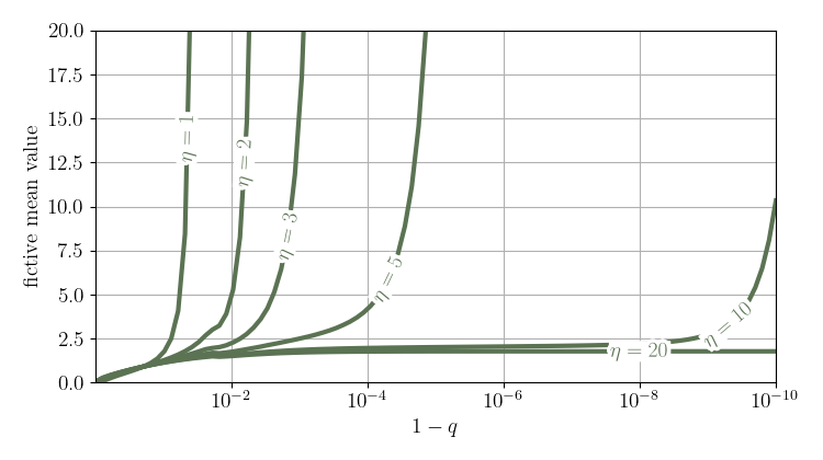
For $\eta \ge 20$, the "fictive" mean has a plateau between $1-10^{-3}$ and $1-10^{-10}$. For $\eta<10$, no such plateau exists. For $\eta=10$, the "fictive" mean explodes if $1-q>10^{-8}$.  ■