How to interpret the outcome of a Monte Carlo simulation if no failures occurred?

If Monte Carlo simulation (MCS) is applied to solve a structural reliability problem, it can happen that none of the samples generated fall into the failure domain. Let $K$ be the total number of samples in a MCS. Furthermore, let $H$ be the number of samples for which $\mathcal{F}$ occurred; i.e., for which $g\left(\mathbf{x}\right)\le 0$. For $H=0$, the point estimate $\widehat{p} = {H}/{K}$ becomes zero, independent of $K$. Structural reliability methods are typically applied to verify that the reliability of the system of interest is larger than a prespecified target reliability. If this verification is based on the point estimate $\widehat{p}$, then $H=0$ is not acceptable, as $\widehat{p} = 0/K$ is misleading.

The outcome $H=0$ is, however, acceptable if a Bayesian post-processing of MCS is applied.  The posterior for $p_f$ can be used to quantify how credible it is that the prespecified target reliability is maintained, even if $H=0$. Therefore, Bayesian post-processing of MCS is of particular relevance, if the reliability of the system of interest is much larger than the prespecified target reliability, as $K$ can be significantly smaller than the number of samples needed to achieve an $H>0$. A (biased) Bayesian point estimate is the expected value of the posterior probability of failure $P_f$. With the maximum entropy prior this estimate is (conditional on $H=0$):
$$
\widehat{p}_\mathrm{Bayes} = \frac{H+1}{K+2} = \frac{1}{K+2}\,,
$$ which is always larger than zero.

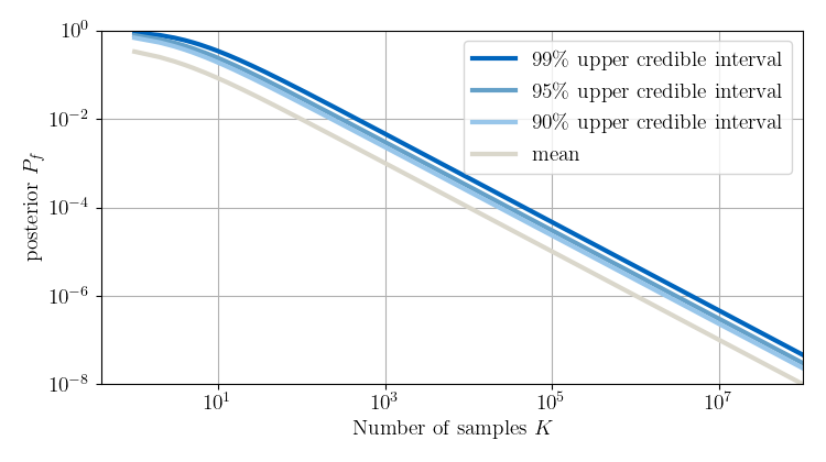
Moreover, based on the posterior distribution for $P_f$, credible intervals can be derived. In the plot above, for $H=0$, the number of samples $K$ needed to achieve the specified credibility for the value of $P_f$ is shown. If, for example, if the aim is to demonstrate that $p_f \le 10^{−6}$, then $K = 3 \times 10^6$ samples are needed to verify that the posterior $P_f$ is smaller than the target with probability 90%, $K = 4 \times 10^6$ samples are needed to verify that the posterior $P_f$ is smaller than the target with probability 95%, and $K = 5 \times 10^6$ samples are needed to verify that the posterior $P_f$ is smaller than the target with probability 99%. The posterior mean for $P_f$ is already smaller than the target for at least $10^6$ samples.

You can quantify the outcome of a MCS by using our Online Tool for post-processing of MCS.