How to use Monte Carlo simulation for reliability analysis?

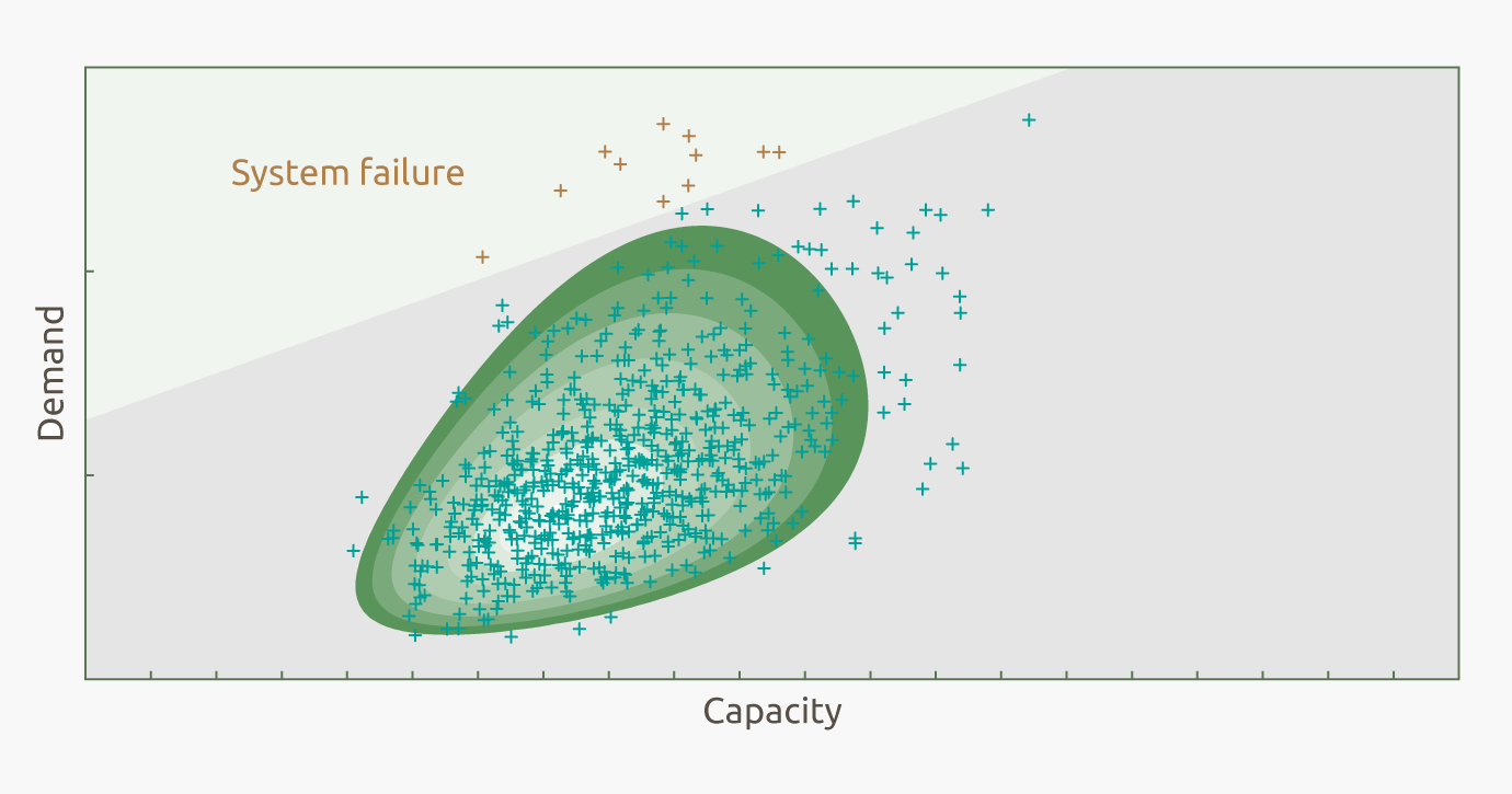
Monte Carlo simulation (MCS) is a simple, straightforward and robust method. The principle steps in a MCS are: (1) A set of random variables $\mathbf{X}$ that follow joint probability density function $f_\mathbf{X}(\mathbf{x})$ is defined. (2) $K$ random samples $\mathbf{x}_{(1)},\ldots,\mathbf{x}_{(K)}$ are generated from $f_\mathbf{X}(\mathbf{x})$. (3) For each sample the response of the underlying model response $h(\cdot)$ is evaluated; i.e., $h_{(i)}=h(\mathbf{x}_{(i)})$. (4) The quantities $h_{(1)},\ldots,h_{(K)}$ are aggregated; e.g., by using the sample mean $\operatorname{E}\left[h(\mathbf{X})\right] \approx \widehat{h} = \frac{1}{K} \sum_{i=1}^K h_{(i)}$.

To apply MCS to structural reliability analysis, we express the integral to evaluate the probability of failure as follows:
$$
p_f = \Pr(\mathcal{F}|\mathcal{M}) = \int_{\Omega} I(\mathbf{x}) f_\mathbf{X}(\mathbf{x}) \, \operatorname{d}\mathbf{x}\,,
$$ where $I(\mathbf{x})$ is an indicator function defined as:
$$
I(\mathbf{x}) =  \begin{cases}
    1   & \text{if } g(\mathbf{x})\le 0 \\
    0   & \text{otherwise}
  \end{cases}\,,
$$ with $g(\mathbf{x})$ as the limit state function.

Note that the above integral to evaluate $p_f$ is equivalent to the expected value of $I(\mathbf{X}) $; i.e., $p_f = \operatorname{E}\left[I(\mathbf{X})\right]$. Thus, a value for the probability of failure $p_f$ can be estimated as follows:

1. Set up a reliability problem by defining the vector of uncertain model parameters $\mathbf{X}$, the joint probability density function $f_\mathbf{X}(\mathbf{x})$ of $\mathbf{X}$ and limit state function $g(\mathbf{x})$.
2. Generate $K$ random samples $\mathbf{x}_{(1)},\ldots,\mathbf{x}_{(K)}$ from $f_\mathbf{X}(\mathbf{x})$.
3. For each sample $\mathbf{x}_{(i)}$, evaluate the limit state function $g(\mathbf{x})$.
4. An unbiased estimate for $p_f$ is obtained by a weighted sum over $K$ samples: $$
   p_f = \operatorname{E}\left[I(\mathbf{X})\right] \approx \widehat{p} = \frac{H}{K}\,,
   $$ with $H = \sum_{i=1}^K I(\mathbf{x}_{(i)})$.

If MCS is employed to estimate small values of $p_f$, typically a very large number $K$ of samples is required to obtain sufficiently accurate results. This often renders MCS computationally infeasible for application in numerical reliability analysis. Especially if the analysis is based on computationally demanding models (e.g., finite element models), the computational burden to evaluate thousands of model runs is typically just too large. However, whenever it is computationally feasible to apply MCS, MCS is the most robust structural reliability method amongst all sampling-based structural reliability methods.

You can use our Online Tool for post-processing of MCS to quantify the uncertainty about the value of $p_f$ based on a conducted MCS.