How large is the statistical uncertainty in the estimate of a Monte Carlo simulation?

In this article, we discuss the statistical uncertainty of the estimated probability of failure $\widehat{p}$ in a Monte Carlo simulation (MCS). The assumption underlying this article is that the actual probability of failure $p_f$ of the system of interest is deterministically known. In a separate article, we discuss the more general and practical relevant case of how to assess the uncertainty in the outcome of a Monte Carlo simulation if $p_f$ is not known deterministically.

Monte Carlo simulation of rare events

In MCS, $K$ independent samples $\mathbf{x}^{(1)},\ldots,\mathbf{x}^{(K)}$ of the input random vector $\mathbf{X}$ are generated and for each sample $\mathbf{x}^{(i)}$ the limit-state function $g\left(\mathbf{x}^{(i)}\right)$ is evaluated. We count the number $H$ of occurrences of the event $\mathcal{F}$, for which $g\left(\mathbf{x}\right)\le 0$, is counted; i.e., $H$ expresses for how many samples the modeled performance of the system of interest is unsatisfactory. An unbiased point estimate $\widehat{p}$ for $p_f$ is obtained as:
$$
p_f \approx \widehat{p} = \frac{H}{K}\,.
$$

Statistical uncertainty of the estimate $\widehat{p}$

$H$ can be perceived as the outcome of a Bernoulli process. Each element in this Bernoulli process of length $K$ is an independent and identically distributed (iid) Bernoulli trial and follows a Bernoulli distribution with a mean value equal to $p_f$. Consequently, the number $H$ of observed failures in a MCS with a total number of $K$ samples is the outcome of a binomial distributed random variable with parameter values equal to $K$ and $p_f$.

As the estimate $\widehat{p}$ is obtained by dividing $H$ by $K$, the variance of $\widehat{p}$ for repeated runs of the MCS with a fixed total number of samples $K$ is:
$$
\operatorname{Var}\left[\widehat{p}\right] = \frac{p_f\cdot (1-p_f)}{K}\,.
$$ The coefficient of variation of $\widehat{p}$ is:
$$
\delta_{\mathrm{MCS}} = \frac{\operatorname{Var}\left[\widehat{p}\right] }{p_f} = \sqrt{\frac{1 - p_f}{p_f \cdot K}}\,.
$$ Even though $\delta_{\mathrm{MCS}}$ depends on the (unknown) underlying $p_f$, the equation above highlights the major strength and weakness of Monte Carlo simulation: On the one hand, the weakness is that for small $p_f$ the total number of samples $K$ must be large to achieve a reasonable coefficient of variation of the estimate. On the other hand, the strength of MCS is that $\delta_{\mathrm{MCS}}$ does not depend on the number of stochastic variables; i.e., the dimension of $\mathbf{X}$.

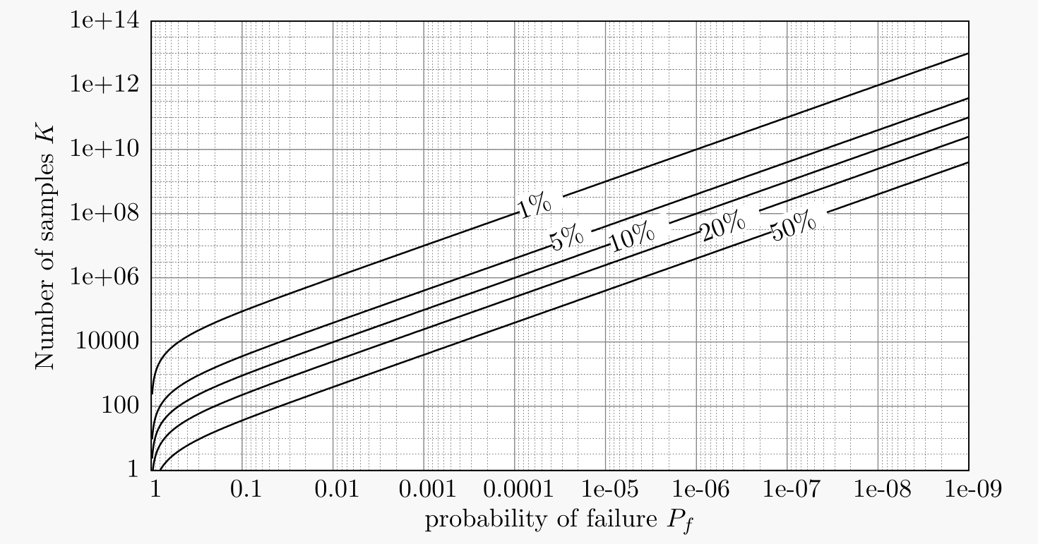
Number of samples required to maintain a target coefficient of variation

The plot on top of this article illustrates the required number $K$ of samples to maintain a specific target coefficient of variation $\delta$ for a given probability of failure $p_f$. The relation underlying the plot above to achieve a $\delta_{\mathrm{MCS}} \le \delta$ can be expressed analytically as follows:
$$
K \ge \frac{1-p_f}{p_f\cdot\delta^2}\,.
$$

Outlook

Both equations above depend on the (unknown) underlying $p_f$. Thus, for the practical application of MCS, these expressions are not optimal to quantify the uncertainty about the value of $p_f$. To fully quantify the uncertainty about the value of $p_f$ in case the value of $p_f$ is not deterministically known in advance, you can use our Online Tool for post-processing of MCS to based on a conducted MCS.